How to Compare Two Columns in Google Sheets (Best 5 Methods)

Key Takeaways:

• Step-by-Step Guide: Learn how to compare two columns in Google Sheets using various formulas, including IF, EXACT, and VLOOKUP, to ensure your data matches accurately.
• Advanced Tool Recommendation: Explore SmartMatchApp for more efficient data comparison and matchmaking, specifically tailored for those in the matchmaking business.

Almost everyone needs to compare two columns in Google Sheets at some point, whether for work, school, or personal projects. But if you’re not using the right techniques, you could miss out on better results. In this article, I’ll show you how to compare two columns in Google Sheets using different formulas. Plus, I’ll introduce you to an even better tool for matching and comparing data later on. So, keep reading—your data deserves the best.

How to Compare Two Columns in Google Sheets Using IF Function

The IF function is one of Google Sheet's most versatile tools, and it’s especially handy when you need to check if two columns match in Google Sheets. This method allows you to return a specified value based on the comparison result, such as indicating "matching values" with "Yes" or "Match" for identical entries.

Step-by-Step Guide

Start by entering the following formula in a new column adjacent to the two columns you want to compare: =IF(A2=B2, "Match", "No Match")

1. Replace A2 and B2 with the appropriate cell references for your data.
2. Drag the Formula Down: Once the formula is in place, drag the fill handle down to apply it to all the cells in the column. This will automatically compare the values in both columns row by row.
   
   
3. Interpret the Results: If the values in both columns match, the cell will display "Match"; if not, it will show "No Match." This method is particularly useful when you need to quickly see if two columns match in Google Sheets.

How to Match Data in Two Columns in Google Sheets Using the EXACT Function

The EXACT function is another powerful tool in Google Sheets that allows you to match two columns, ensuring that every detail is identical, including case sensitivity. This function helps in identifying matching data cells across the columns' rows, making it easier to see which cells correspond with each other.

Step-by-Step Guide

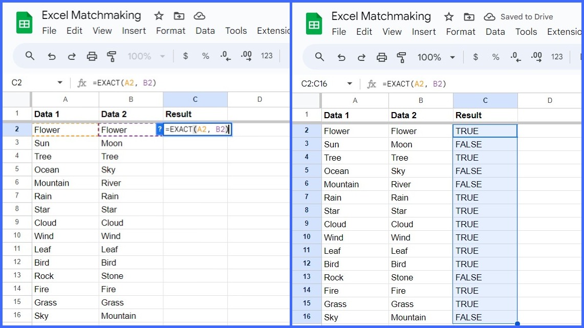
In a new column, enter the following formula: =EXACT(A2, B2)

1. Replace A2 and B2 with the cell references of the columns you want to compare.
   
   
2. Drag the Formula Down: Drag the fill handle down to apply the formula across the column. This will help you check if two columns match in Google Sheets, considering every detail.
   
   
3. Interpret the Results: The formula returns TRUE if the values in both columns match exactly, and FALSE if they differ in any way. This method is particularly useful when you need to ensure that every aspect of your data is consistent across columns.

How to Check if Two Columns Match in Google Sheets with Conditional Formatting

Conditional formatting provides a visual method to compare two columns in Google Sheets by highlighting differences, matches, or duplicate values.

Step-by-Step Guide

1. Select the Data: Highlight the cells in the first column that you want to compare.
   
   
2. Apply Conditional Formatting: Go to the Home tab, click on Conditional Formatting, and choose New Rule.
   
   
3. Create a Formula Rule: Select Use a formula to determine which cells to format, and enter the following formula: =A2<>B2
   
   
4. Choose a formatting style, like a fill color, and click OK.
   
   
5. Drag the Formatting Across the Column: Apply the same conditional formatting to the entire column. This method provides a quick visual cue to tell if two columns match in Google Sheets or not.

How to Match Up Two Columns in Google Sheets Using the VLOOKUP Function

The VLOOKUP function is another robust tool that helps you compare two columns by looking up values in column B and returning a match or an error.

Step-by-Step Guide

In a new column, enter the following formula: =VLOOKUP(A2, $B$2:$B$100, 1, FALSE)

1. Replace A2 with the cell reference from the first column and $B$2:$B$100 with the range of cells in the second column.
   
   
2. Drag the Formula Down: Drag the fill handle down to apply the formula across the column. This will help you match data in two columns in Google Sheets and return the corresponding value if a match is found.
   
   
3. Interpret the Results: If the value in the first column exists in the second column, VLOOKUP will return that value. If not, it will return an #N/A error. This method is especially useful when you need to compare if two columns match in Google Sheets using a simple and efficient approach.

How to Match Values in Two Columns in Google Sheets Using the MATCH Function

The MATCH function is perfect for finding the relative position of a value in a specified range. When combined with the IF function, it becomes a highly effective way to check if two columns contain matching data in Google Sheets. If you want to learn more about how to match in excel with match and index functions, read our full article on that here.

Step-by-Step Guide

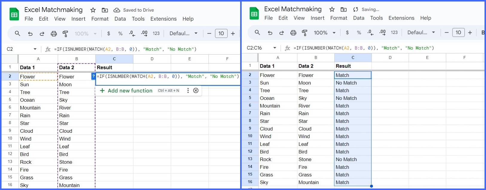
In a new column, enter the following formula: =IF(ISNUMBER(MATCH(A2, B:B, 0)), "Match", "No Match")

1. Replace A2 with the cell reference from the first column.
   
   
2. Drag the Formula Down: Drag the fill handle down to apply the formula across the column. This method helps you easily identify if values in two columns match in Google Sheets by finding their relative positions.
   
   
3. Interpret the Results: This formula returns "Match" if the value in the first column is found anywhere in the second column and "No Match" if it isn’t. This technique is highly effective for quickly checking if two columns match in Google Sheets, especially when working with large datasets.

Why SmartMatchApp is a Better Alternative for Matchmaking

While Google Sheets provides several methods to compare two columns, it might not be the best fit for those in the matchmaking business, where efficiency and accuracy are paramount. Manually comparing columns in Google Sheets is often a tedious and time-consuming process, especially when dealing with large and linked spreadsheets. If you’re constantly comparing data to find the perfect matches—whether for business partnerships, professional networking, or personal relationships—consider a tool designed specifically for this purpose. SmartMatchApp offers a streamlined solution that automates the matching process, saving you time and reducing the potential for errors.

How SmartMatchApp Simplifies Data Comparison

Unlike Google Sheets, where you need to manually set up and tweak formulas, SmartMatchApp automates the entire process. Simply input your criteria, and SmartMatchApp will handle the rest, delivering precise matches in seconds. It efficiently identifies matching or mismatching data, ensuring that no potential match is overlooked. Whether you’re dealing with a few dozen or thousands of entries, SmartMatchApp processes your data efficiently. This tool is tailored for matchmakers who need to compare and connect people or businesses, making it the perfect alternative to Google Sheets for this type of work. You wanna see how it works? Get SmartMatchApp free trial here!

Conclusion

Comparing two columns in Google Sheets doesn’t have to be a daunting task. Identifying the same data between columns is crucial for data comparison tasks, as it helps in highlighting duplicates or unique entries. Whether you’re using simple functions like IF and EXACT or leveraging more advanced techniques like VLOOKUP and PivotTables, Excel offers a variety of tools to help you efficiently compare and analyze your data.

By mastering these methods, you can streamline your data management process, ensure accuracy, and make your workflow more efficient. Whether you’re comparing small lists or large datasets, these techniques will help you get the job done with precision and ease.

And if you’re in the business of making connections and need a tool that’s specifically designed for matchmaking, SmartMatchApp is the ideal alternative. It takes the hassle out of manual data comparison, giving you more time to focus on what really matters—building meaningful connections.

Frequently Asked Questions

Let's answer some frequently asked questions.

How to compare two columns in Google Sheets?

To compare two columns in Google Sheets, follow these steps:

• Step 1: Enter the formula =IF(A2=B2, "Match", "No Match") in a new column next to the columns you want to compare.
• Step 2: Replace A2 and B2 with the correct cell references for your data.
• Step 3: Drag the fill handle down to apply the formula to all rows.

This will show "Match" if the values are the same, or "No Match" if they differ.

Can you compare two columns in Google Sheets using the Index-Match function?

Yes, you can compare two columns in Google Sheets using the Index-Match function. The INDEX-MATCH combination is a powerful tool that allows you to match entries between two different tables and pull corresponding values. For example, if you're comparing the data in Column D with Column A, the MATCH function will find the position of matching values, and the INDEX function will then pull the corresponding data from another column. If there's no match, it will return #N/A.

How to compare three or more columns in Google Sheets?

To compare three or more columns in Google Sheets and find matches, you can use the IF function combined with the AND statement. This method checks whether all cells in the specified columns match. For instance, the formula =IF(AND(A2=B2, A2=C2), "Full match", "") will return "Full match" if the values in Columns A, B, and C are identical in the same row. If you want to find matches in any two cells within the same row, you can use the OR statement: =IF(OR(A2=B2, B2=C2, A2=C2), "Match", ""). This formula will return "Match" if any two of the three cells have the same value.